Page Comparison

...

This pipeline is available in https://utap.wexac.weizmann.ac.il/. 

Before you start:

This pipeline runs on the Wexac cluster. 
Please prepare the following in advance:

1. An account (userID) on Wexac, via your department administrator.
2. A "Collaboration" folder within your lab folder on Wexac, with read and write permission for Bioinformatics Unit staff. This must be set up by the computing center (hpc@weizmann.ac.il).
3. Sufficient free storage space on Wexac (> 400Gb), via your department administrator.

In order to run a new transcriptome ATAC-seq analysis, you must first transfer demultiplexed sequencing data (fastq files) to your Collaboration folder. Within the Collaboration folder, a directory structure will be created supporting with outputs of the transcriptome analysis setup described below.

Setting up a new analysis

...

Fastq file name conventions: Fastq file names must start with the same sample name as the subfolders, and end with "_R1.fastq"  (or "_R1.fastq.gz") for single-read data . In the case of paired-end data, corresponding files must exist that are IDENTICAL in their name, but contain the suffix "_R2.fastq" (or "_R2.fastq.gz") instead of "_R1.fastq", where R is the read number.

For example:

• root_folder 
• sample1
  
  • sample1_R1.fastq
  • sample1_R2.fastq (must exist in paired-end)
    Or:
  • sample2_R1.fastq.gz
  • sample2_R2.fastq.gz (must exist in paired-end)
• sample1
• sample2

The pipeline also support supports the fastq file format conventions  _S*_L00*_R1.fastq or _S*_L00*_R1_0*.fastq.

For example:

• root_folder 
• sample1
  
  • sample1_S0_L001_R1_001.fastq
  • sample1_S0_L001_R1_002.fastq
  • sample1_S0_L002_R1_001.fastq
  • sample1_S0_L002_R1_002.fastq
  • sample1_S0_L001_R2_001.fastq (must exist in paired-end)
  • sample1_S0_L001_R2_002.fastq (must exist in paired-end)
  • sample1_S0_L002_R2_001.fastq (must exist in paired-end)
  • sample1
_S0_L002_R2_002.fastq (must exist in paired-end)
• sample2_S0_L001_R1_001.fastq
• sample2_S0_L001_R1_002.fastq
• sample2_S0_L002_R1_001.fastq
• sample2_S0_L002_R1_002.fastq
• sample2_S0_L001_R2_001.fastq (must exist in paired-end)
• sample2_S0_L001_R2_002.fastq (must exist in paired-end)
• sample2_S0_L002_R2_001.fastq (must exist in paired-end)
sample2
• • _S0_L002_R2_002.fastq (must exist in paired-end)
• sample1
• sample2

UTAP user interface input information required: 

...

For mouse, you have the option to choose a TSS file, containing either a broad or narrow definition of the genes’ TSS (Transcription Start Site) regions (based on <Author et al>, Nature. 2016 Jun 30;534(7609):652-7 - The landscape of accessible chromatin in mammalian preimplantation embryos).

...

Finally, click the “Run analysis” button to submit the analysis. Once the analysis is completed, you will be notified by email (usually after a few hours).
All of the output files will be stored in your Wexac Collaboration folder.
At this point no report is being created.

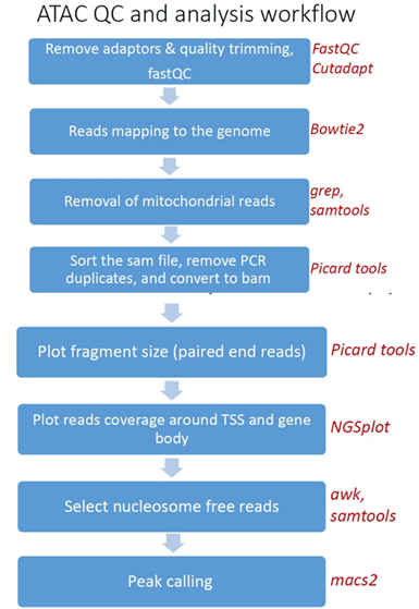
Analysis workflow

Pipeline steps and associated tools:

1. Quality controlReads trimming: Reads are quality trimmed using cutadapt. In this process primers corresponding to the TruSeq protocol are removed (output is in folder 1).
2. Quality control: Reads quality control is evaluated using FastQC (in output folder 2), and a report file, containing quality reports for all of the samples, is generated using multiQC (in output folder 3).
3. Mapping to genome: The quality trimmed paired-end reads are mapped to Mouse/Human genomes using Bowtie2 (output is in folder 4).
4. Alignment filtering: Following the alignment, mitochondrial genes are removed from the analysis (using the grep command). Duplicated reads are removed using picard-tools. The remaining unique reads are indexed and sorted using samtools index and samtools sortGenerate statistics . Statistics on the alignment is generated using flagstat (output is in folder 5).
5. Select nucleosome-free fragments: fragments of length <120bp are selected using the awk command (alignments are in folder 6), and insert size distributions are plotted before and after size selection (output is in folder 8, plots after selection end with "_nucl_free").
6. Visualization in graphs: The analyzed reads reads coverage on gene body and around the TSS are graphically visualized using ngsplot .Select nucleosome-free fragments: fragments of length <120bp are selected(output is in folder 7).
7. Read counts on TSS: for mm10 genome we count the number of reads on genes’ TSS (Transcription Start Site) regions based on, Nature. 2016 Jun 30;534(7609):652-7 ).
8. Peak calling: Peaks Broad peaks are called using MACS2 (output is in folder 10).

Output folders:

1_cutadapt

...

4_mapping

5_process_alignment

6_nucleosome_free

7_ngs_plot7

8_nucleosomepicard_freeplot

89_tss_count

910_call_peak

1011_reports

Log files (one directory above the output directory):

...