UTAP: ChIP-seq pipeline guidelines
Pipeline website: https://utap.wexac.weizmann.ac.il/
The CHIP-seq (Chromatin Immunoprecipitation followed by Sequencing) pipeline facilitates the analysis of CHIP-seq data in order to identify genome-wide DNA binding sites for transcription factors and other proteins. The pipeline receives single or paired-end reads as input (the type of input is automatically determined by the number of fastq files generated per sample), performs quality control and pre-processing steps, and maps the reads onto mouse or human genomes. Peak analysis is then performed (after some post-processing), on the identified DNA binding fragments, and significant peaks (as compared to a control background if present) are selected and analyzed.
Before you start:
This pipeline runs on the Wexac cluster.
Please prepare the following in advance:
- An account (userID) on Wexac, via your department administrator.
- A "Collaboration" folder within your lab folder on Wexac, with read and write permission for Bioinformatics Unit staff. This must be set up by the computing center (hpc@weizmann.ac.il).
- Sufficient free storage space on Wexac (> 400Gb), via your department administrator.
In order to run a new transcriptome analysis, you must first transfer demultiplexed sequencing data (fastq files) to your Collaboration folder. Within the Collaboration folder, a directory structure will be created supporting the transcriptome analysis setup described below.
Setting up a new CHIP-seq analysis
If you wish to run a new CHIP-seq analysis from existing files in the Collaboration folder, or if you’ve uploaded new sequencing data (not produced within the LSCF) to Wexac from an external source, login to ngsbio.wexac.weizmann.ac.il via Firefox or Chrome (the pipeline is NOT compatible with Internet Explorer) using your Weizmann userID and password.
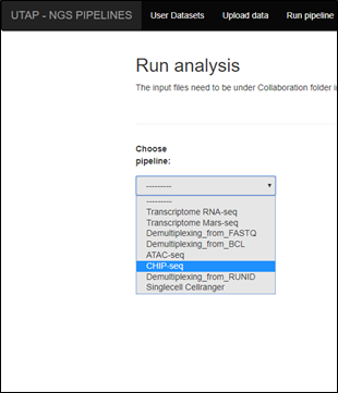
- Click on CHIP-seq pipeline in the choose pipeline box:
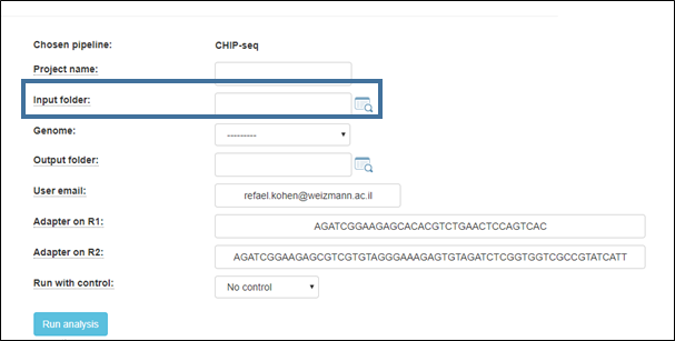
2. Select the input folder:
Browse within your Collaboration folder and select the folder containing your sample files (fastq). Fastq files must be organized, within the selected folder (depicted as root folder in the example below), into subfolders as shown below.
Note that if you wish to go up one level (or more), click the desired folder level on the path at the top of the window.
Fastq file name conventions: Fastq file names must start with the same sample name as the subfolders, and end with "_R1.fastq" (or "_R1.fastq.gz") for single-read data. For paired-end data, corresponding files must exist that are IDENTICAL in their name, but contain the suffix "_R2.fastq" (or "_R2.fastq.gz") instead of "_R1.fastq", where R is the read number.
For example:
- root_folder
- sample1_R1.fastq
- sample1_R2.fastq (must exist in paired-end)
- sample2_R1.fastq.gz
- sample2_R2.fastq.gz (must exist in paired-end)
- sample1
- sample2
The pipeline also supports the fastq file format conventions _S*_L00*_R1.fastq or _S*_L00*_R1_0*.fastq.
For example:
- root_folder
- sample1_S0_L001_R1_001.fastq
- sample1_S0_L001_R1_002.fastq
- sample1_S0_L002_R1_001.fastq
- sample1_S0_L002_R1_002.fastq
- sample1_S0_L001_R2_001.fastq (must exist in paired-end)
- sample1_S0_L001_R2_002.fastq (must exist in paired-end)
- sample1_S0_L002_R2_001.fastq (must exist in paired-end)
- sample1_S0_L002_R2_002.fastq (must exist in paired-end)
- sample2_S0_L001_R1_001.fastq
- sample2_S0_L001_R1_002.fastq
- sample2_S0_L002_R1_001.fastq
- sample2_S0_L002_R1_002.fastq
- sample2_S0_L001_R2_001.fastq (must exist in paired-end)
- sample2_S0_L001_R2_002.fastq (must exist in paired-end)
- sample2_S0_L002_R2_001.fastq (must exist in paired-end)
- sample2_S0_L002_R2_002.fastq (must exist in paired-end)
- sample1
- sample2
3. Select the output folder
If you want the output folder to be different from the one automatically filled in (based on the selected input folder), overwrite the output folder name in the text box associated with the screen’s Output folder: field with your name of choice. Additional setups
Fill in a project name, and select the reference genome to which the reads will be aligned.
Default adapters are the P5 and P7 adapters of the Tru-seq protocol.
4. Run with control
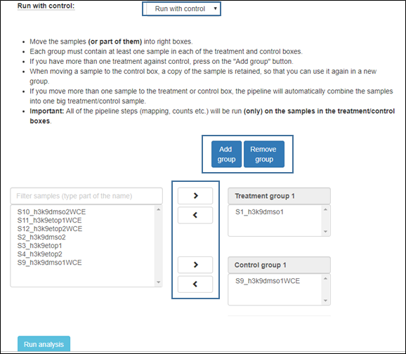
Choose “run with control” in order to compare each treatment to its corresponding control. When selecting this option, a new group of control and treatment boxes will open. Organize the samples by selecting them and using the arrows to move to the appropriate categories.
If you have more than one treatment against control, press on the "Add group" button as shown in the figure below.
Each group must contain at least one sample in each of the treatment and control boxes.
When moving a sample to the control box, a copy of the sample is retained, so that you can use it again in a new group.
If you move more than one sample to the treatment or control box, the pipeline will automatically combine the samples into one big treatment/control sample.
Important: All of the pipeline steps (mapping, counts etc.) will be run (only) on the samples in the treatment/control boxes.
5. Run the pipeline
Finally, click the “Run analysis” button to submit the analysis. You will be notified by email when the analysis is ready (usually after a few hours). All of its output files will be stored in the relevant subfolders within your Wexac Collaboration folder.
Analysis workflow
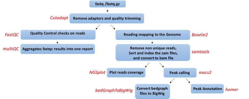
Pipeline steps and associated tools:
- Quality control: Reads are trimmed using cutadapt (DOI: 14806/ej.17.1.200) (with the parameters --times 2 -q 20 -m 25). In this process, primers corresponding to the Tru-seq protocol are removed.
- Quality control: Reads quality control is evaluated using FastQC (with the parameter --cassava). A report file, containing quality results for all of the samples is generated using multiQC.
- Mapping to genome: The quality trimmed reads a mapped to Mouse/Human genomes: /shareDB/iGenomes/Mus_musculus/UCSC/mm10/Sequence/Bowtie2Index/genome /shareDB/iGenomes/Homo_sapiens/UCSC/hg19/Sequence/Bowtie2Index/genome, /shareDB/iGenomes/Homo_sapiens/UCSC/hg38/Sequence/Bowtie2Index/genome respectively, using Bowtie2 (doi: 10.1038/nmeth.1923.) (with the parameters --local for all analyses and, in addition, -X 2000 for paired end analyses). Refseq annotation is provided for the mapped genes.
- Following the alignment, duplicated reads are removed using samtools view (with the parameters -h -F 4 for all reads and, in addition, -f 0x2 for paired end reads). The remaining unique reads are indexed and sorted using samtools index and samtools sort
- Generate statistics on the alignment using flagstat.
- Visualization in graphs: The reads are graphically visualized using ngsplot (with the parameters -G -R genebody -C -O samples -D refseq -L 50000).
- Peak calling: Significant chip regions (peaks) are evaluated and compared to control samples if present using macs2 callpeak (with the parameters --bw 300 -B -f --SPMR -g -keep-dup auto -q 0.01 for all analyses, BAMPE --nomodel for paired end analyses, and BAM for single end analyses).
- Convert to BigWig format: Files containing the predicted peaks coordinates in BedGraph format are converted to BIgWig format using bedtools slop (with the parameters -g -b 0), bedClip stdin and bedGraphToBigWig (with default parameters)
- Peak annotation: The peaks were merged using FILL IN and were annotated according to the corresponding genome using Homer (with default parameters).
Output folders:
1_cutadapt
2_fastqc
3_multiQC
4_alignment
5_samtools
6_peaks_prediction
7_peaks_annotation
8_graphs
9_BigWig
Log files (stored one directory above the output directory)
snakemake_stdout.txt (stored one directory above the output directory)


